In the Coverage step you can explore and edit your coverage results with dedicated tools. The default screen displays the coverage for one or several coverage pairs. But you can examine coverage for additional image pairs, and display a summary of all your results. If you analyze several gels and/or blots in the same experiment, you can go beyond the simple reporting of coverage to explore the presence/absence of individual protein spots across all images.

How to

Discover the Coverage screen

Coverage tabs

By default, you will see two or more tabs at the top of the screen:

• A Coverage summary tab, where you can create and manage additional pairs for coverage analysis. It also summarizes the coverage results for selected coverage pairs.
• A tab for the coverage analysis of the current image pair.
• A tab for the coverage analysis of additional image pairs, if your experiment includes at least two secondary images.

There will be an additional tab for each newly opened coverage analysis. Clicking a tab will show the coverage results for the corresponding image pair, organized into the following screen areas.

Display area

The Display area shows the two images of your image pair. In principle:

• The primary image, at the left, represents the total protein content of the HCP antigen.
• The secondary image, at the right, reveals the proteins detected with the anti-HCP antibody.

At the right of the Display area, you will find the standard Toolbar to manipulate the image views, and set the visualization options.

The spots on these two images are color-coded according to their coverage Status (see below).

Coverage table

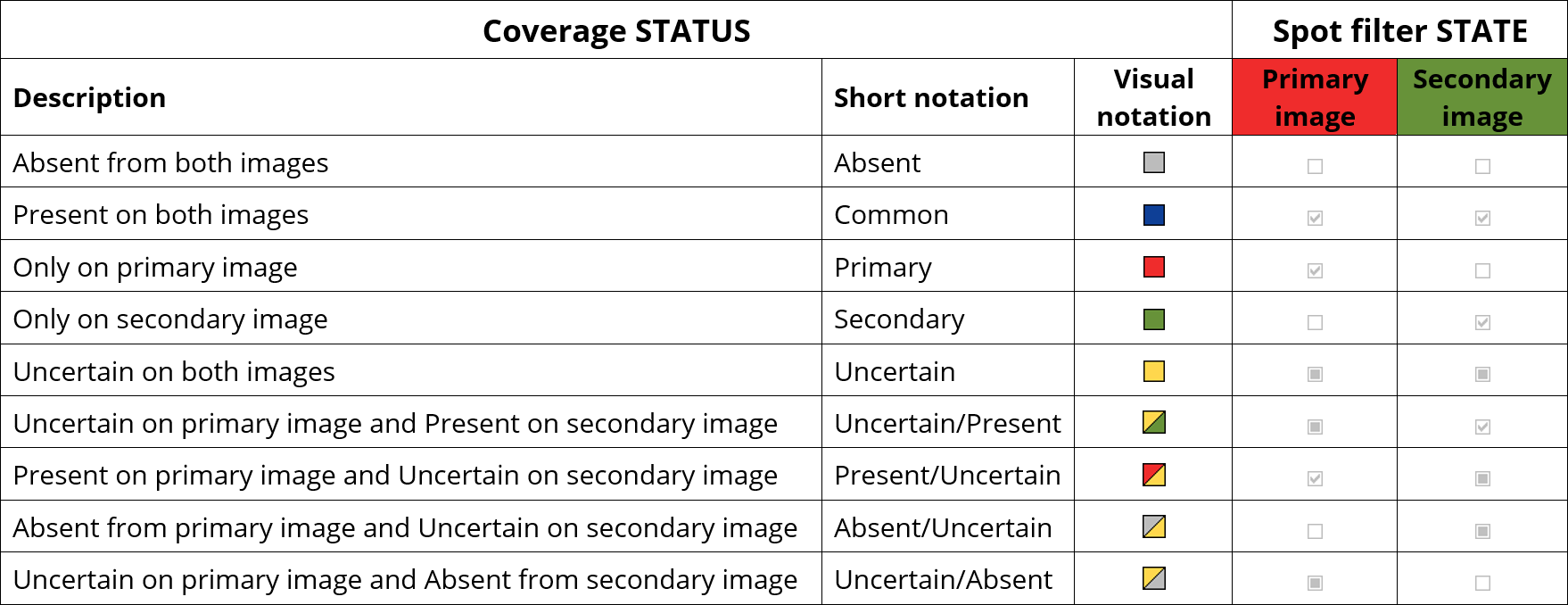
The Coverage table lets you view and edit a spot’s coverage Status as a colored square. The software automatically assigns this status based on the output of the presence filter in the previous step. Indeed, based on the quantitative filters, every spot was assigned a State on each image:

• Absent
• Present
• Uncertain

The spot’s state on the primary image is displayed in the P:State column in the Coverage table (P for Primary image). Similarly, the spot’s state on the secondary image is displayed in the S:State column (S for Secondary image). The table also displays the spot’s Intensity and Volume for each image.

Melanie determines the default coverage status based on the following combinations of the spot states (in the last two columns).

Notes

Manually edited spots are an exception to the above rules. Such spots are always showing a default uncertain status, regardless of the spot’s filter states.

All spots with a yellow component in their coverage status are displayed as uncertain (yellow) on the images and in the Coverage diagram.

The default coverage status can be reviewed and edited. When a spot’s automatically assigned presence status was modified subsequent to spot editing or a user edit, a tick mark is shown in the Status edited field in the Coverage table.

Coverage

Melanie uses the status of all qualified spots to calculate the Coverage for your image pair, i.e. the percentage of immunodetection that the antibody reagent offers for the total population of HCPs. In the Coverage tab of the General Options, you can choose how Melanie calculates the coverage (for each of the three possible coverage types):

• Intersection vs Primary image spots:

Coverage = (Common) / (Primary + Common)

• Secondary vs total number of spots:

Coverage = (Common + Secondary) / (Primary + Common + Secondary)

• Intersection vs total number of spots:

Coverage = (Common) / (Primary + Common + Secondary)

TIP

This last option is equivalent to the Jaccard similarity coefficient. Use it to measure the similarity between two primary images or two secondary images.

NOTE

The formulas above show that the calculated coverage does not consider spots with an uncertain status. Therefore, the coverage is tentative while there are uncertain spots. When you review the uncertain spots and assign them an appropriate status, percent coverage will be updated.

The coverage is reported in the Coverage diagram.

Coverage range

To avoid the subjectivity of spot status editing, integrate the notion of uncertainty in your results or simply save time, you can report the Coverage range instead of the coverage. The coverage range indicates the interval within which your coverage will lie if you only edited the spots with uncertain state, considering that each such spot could either be absent or present. It is displayed in brackets after the coverage percentage, only for as long as there are uncertain spots.

The coverage range can help you gauge the stability and robustness of your coverage analysis and tells whether a detailed spot review is relevant. If, before review of uncertain spots, the coverage range is

• small, e.g. 5-10% interval:  You can be relatively confident about the results and consider a detailed spot review.
• large, e.g. 20-30% interval: You better first determine what causes the large interval. Do you have any issues with the experiment, detection modalities, image acquisition, alignment, detection parameters or presence filter thresholds?

NOTE

If you edit qualified spots as well, your final coverage may fall outside the initially reported coverage range (which only considers uncertain spots).

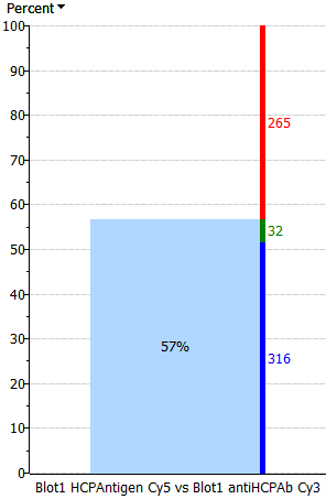
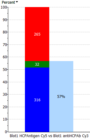
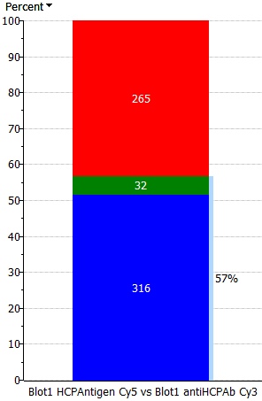
Coverage diagrams

You can visualize the coverage for your image pair, including its calculation and the coverage range, using one of the following options:

Venn diagram	Spot count	Histogram
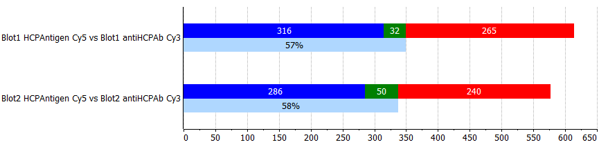
The Venn diagram is most useful as a color-coded legend. It does not bring out the relative number of spots for each status.	The Spot count most effectively conveys the relative number of spots for each status.	The Histogram shows the number of spots for each status on the left, and the percent coverage as a proportional light blue bar on the right. The coverage range is shown as a black vertical interval.

All three coverage diagrams are interactive. You can click on the numbers in the colored areas to select the corresponding spots on the images and in the Coverage table. Clicking on one of the image names at the top of the diagram selects all the spots considered present on that image.

Review status

The Review status section offers various options and tools to simplify review of coverage status.

Show spots

Choose which spots you want to visualize on the images, by selecting an option in Show spots that are:

• All – Shows all spots
• Qualified – Only shows spots with Primary, Common or Secondary status
• Unqualified – Only shows spots with Uncertain status
• On both images – Only shows spots with Common status
• On primary image – Only shows spots with Primary status
• On secondary image – Only shows spots with Secondary status
• Product – Only shows Product spots

Your choice will determine what spots are shown on the images and in the Coverage table. This is useful when reviewing Unqualified spots for instance.

Display

• Show coverage table – Show or hide the coverage table
• Show targeted coverage table – Show or hide the targeted coverage table
• Select spot set – Select all spots from a given spot set
• Select annotated spots – Select all spots from a given annotation category

Edit

• Reset spot qualification – This will reset all status assignments to the default (based on Presence filter output). All user edits of coverage status will be lost.
• Swap images for coverage calculation – This will calculate coverage for the same image pair, but considering the right image as the Primary image, and the left image as the Secondary image. The image positions or colors will not be switched, and the coverage diagram will remain the same. Only the percent coverage and its formula will change. You will be made aware of the switch with the * that will appear after the coverage.

Edit coverage status

Click the Edit coverage status icon to quickly enter the Coverage mode. You can then edit the coverage status by simply clicking on a spot, both in 2D and 3D view. You can also activate the Coverage mode via the Toolbar.

Review coverage status

Uncertain spots

If you used two thresholds in your presence filters, you will have a number of spots that have been tagged uncertain. You can quickly review these spots to assign them an appropriate coverage status and allow calculation of a final percent coverage. The number of uncertain spots to be reviewed appears in yellow in the Coverage diagram.

When reviewing a spot’s coverage status, you must select one of the four options:

• Primary – The spot is only present on the primary image
• Secondary – The spot is only present on the secondary image
• Common – The spot is present on both images
• Absent – The spot is absent from both images

To prepare for efficient coverage status review:

• Show only Unqualified spots in Review status, so you can concentrate solely on the uncertain spots.
  
• Activate the Coverage mode.
• Change to 3D view, because this will allow you to better judge whether a spot is present on an image or not.

TIPS

Use a mouse with a scroll wheel to avoid frequent mode changes to move, zoom and rotate images or increase peak height in 3D view. You will appreciate the simplicity and time savings of using the scroll wheel to manipulate your images.

The default peak heights in the 3D view may give you the impression that many spots are absent. When you increase the peak height however, you will often find that there is a real protein signal. So it is important to adjust the peak height properly. At any moment, you can increase or decrease the peak heights in the 3D view by rolling your mouse scroll wheel while holding the Ctrl key.

You can review and edit coverage status in two ways:

• Click on a spot in one of the images and then select the appropriate coverage status from the four-color tile. You can select several spots by drawing an area over them, or by using the Shift or Ctrl keys. The chosen coverage status will be applied to all selected spots. The spot(s) remain(s) selected and visible until you select the next spot.

• Select a spot in the Coverage table, click on the colored square and choose the appropriate coverage status from the four-colored tile. Once this is done, the spot disappears from the table and the image, and the next spot will be selected for review.

Presence plot

The Presence plot is useful to check if coverage status edits are reasonably coherent with the thresholds set in the Presence filter. Learn more about the Presence plot.

All spots

After reviewing the uncertain spots, it is good practice to do a rapid visual inspection of all spots on your images. Indeed, when spots contain artefacts or are partly overlapping with other spots, their spot value (intensity or volume) may be exaggerated. As a result, some spots may have been labeled present whereas they are absent in reality. On the other side of the spectrum, spots that are saturated cannot be correctly quantified. They can have spot values close to zero and therefore be labeled absent.

To do this quick check on all spots, show All spots in Review status. If you find obvious inconsistencies, you can edit the coverage status as explained above.

All coverage pairs

Once you reviewed your current coverage pair, you can switch tabs to review coverage status on your other image pairs as well.

All spots across all images

Use the Presence summary to review and edit spot presence while visualizing all images.

Define and manage coverage quadrants and targets

Instead of calculating coverage for all spots in your images, you can look at the coverage for a specific subset of spots:

Coverage quadrants

To evaluate the coverage of your antibody for different charge and size categories of proteins, you can create coverage quadrants by specifying pI and MW thresholds. You will instantly see in what pI and MW ranges the antibody coverage is suboptimal and further optimization of immunization strategies is needed.

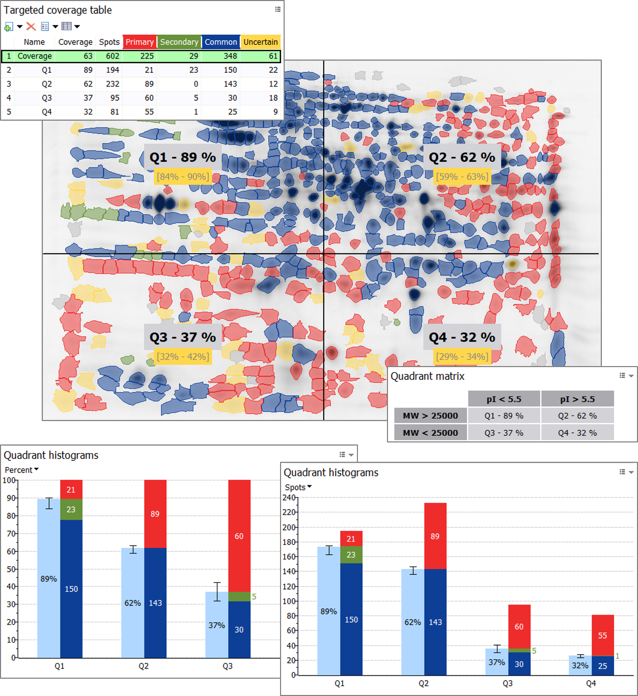
Besides showing the quadrant limits on the images, the feature lets you display the name, coverage percentage and coverage range for each quadrant. The Quadrant histograms and Quadrant matrix complement the results and can be exported as any other graphical report. Since coverage range is assessed for individual quadrants, you’ll know where to best start reviewing uncertain spots to quickly refine your coverage percentage; just select the quadrant with the largest coverage range (black vertical interval) when the Quadrant histograms’ Y-axis is expressed in Percent. In the above example, reviewing the uncertain spots in Q3 will potentially have most impact on percent coverage.

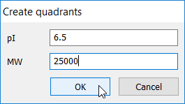
To create or edit quadrants, click the Create targeted coverage icon in the Targeted coverage table and choose Create quadrants. Then enter a pI and MW value in the Create quadrants window.

NOTE

pI and/or MW markers must be defined to use this feature.

If you don’t want to set a threshold for either pI or MW, enter the value -1 or 0.

• If pI and MW thresholds are entered, 4 quadrants are created, named Q1, Q2, Q3 and Q4.
• If only a pI threshold is entered, 2 vertical sections are created, named Low pI and High pI.
• If only a MW threshold is entered, 2 horizontal sections are created, named Low MW and High MW.

To remove the quadrants, click the Remove targeted coverage icon in the Targeted coverage table and select at least one of the quadrants.

To keep your quadrants but temporarily hide the complementary reports or hide the quadrant limits, quadrant names, coverage percentages and coverage ranges from the Display area click the Table icon in the Targeted coverage table:

• Quadrant histograms – Show/hide the Histograms for each quadrant or section. To choose whether the vertical axis in the Quadrant histograms should display Percent or Spots, click on the axis label.
• Quadrant matrix – Show/hide an exportable table that summarizes the coverage for each quadrant and integrates the pI and MW thresholds.
• Display quadrant separations – Show/hide the quadrant separations in the Display area.
• Display quadrant labels – Show/hide the quadrant labels in the Display area.
• Display quadrant coverage percentages – Show/hide the quadrant coverage percentages in the Display area.
• Display quadrant coverage ranges – Show/hide the quadrant coverage ranges in the Display area.

NOTE

Quadrant limits, as well as the quadrant names, coverage percentages and coverage ranges are not displayed in 3D view.

TIP

When you select a quadrant in the Targeted coverage table, only the spots from this quadrant are shown on your images. And the Coverage diagram shows the coverage for the selected quadrant.

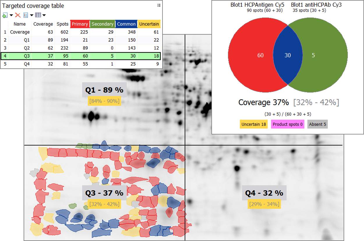
Coverage target from selection or spot set

Alternatively, you can calculate the coverage for a current spot selection or a spot set, also called a Target. If you ran replicate blots for instance, you may want to calculate coverage only for those spots that were detected on both blots, selected using the Presence summary. But you can essentially calculate coverage for any subset of spots, either picked manually or selected through a filter.

NOTE

Spot selection, manually or via Filter by values, only acts on spots shown on the images and in the Coverage table. So when selecting spots in the Coverage step, make sure to show All in Review status. While absent or uncertain spots are not considered in the coverage calculation, it is better to include them in your selection. This way, they will be taken into account in case you change their status.

Use the icons in the Targeted coverage table to manage your targets:

Create targeted coverage – Define a new target for coverage calculation. You can:

• Create targeted coverage from spot selection, if you have spots selected.
• Create targeted coverage from spot set, if you previously defined a spot set.

Remove targeted coverage – Remove existing targets by selecting them from a list.

When you select a target in the Targeted coverage table, only the spots from this target are shown on your images. And the Coverage diagram now shows the coverage for the selected target.

Create and manage additional coverage pairs

Coverage pairs

The Coverage summary table in the Coverage summary tab shows a list of one or several coverage pairs. If you only have 2 images in your project, you will see a single image pair (row) and no additional pairs can be created. If you have more than 2 images in your project, there will be one pair (row) for each secondary image against its corresponding primary image. But you can create and manage additional coverage pairs. You may, for instance, compare the two primary images, or the two secondary images.

Click New to create an additional coverage pair. Select one or several pairs (hold the Shift or Ctrl keys) from the Add new coverage pairs to compare window. The new coverage pairs open in new tabs and will be added to the Coverage summary table.

To delete a coverage pair, select it in the Coverage summary table and click Delete.

Click Properties to view and edit the Name and Note of a selected coverage pair.

Summary columns

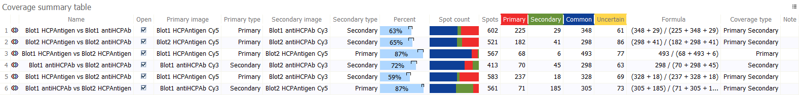
Click the Options icon at the top right of the Coverage summary table and then choose Column settings. Tick all the fields to take a look at the information you can display:

• Name – The name of the coverage pair. You can edit this name by clicking the Properties button.
• Open – Tick or untick this box to show/hide your coverage pair from the Coverage summary histograms and the tabs.
• Primary image, Secondary image – The names of the primary and secondary images.
• Primary type, Secondary type – The types of the primary and secondary images, as they were defined in the Quality control step.
• Coverage – The coverage, on a colored background.
• Percent – The coverage, expressed as a bar proportional to the cell width, for a quick coverage comparison between pairs.
• Spot count – The spot counts as bars proportional to the cell width. The included spot statuses depend on the formula used to calculate coverage.
• Spots – The total number of spots considered in the coverage calculation. It equates the denominator of the formula used to calculate coverage.
• Primary, Secondary, Common, Uncertain – The number of primary, secondary, common and uncertain spots.
• Coverage type – The coverage type of the pair.
• Formula – The formula used to calculate coverage. You can choose it in the Coverage tab of the General options, for each of the three coverage types.
• Note – You can add a description of your coverage pair by clicking the Properties button.

Coverage types

Each pair has one of the following Coverage types:

• Primary Secondary – Compares a secondary image (e.g. anti-HCP antibody) against a primary image (e.g. HCP antigen). The default pairs created are of this type.
• Primary – Compares two primary images (e.g. two HCP antigen replicates).
• Secondary – Compares two secondary images (e.g. two anti-HCP antibody images).

TIP

You will likely want to use different coverage formulas for these coverage types. Whereas the options Intersection vs Primary image spots or Secondary vs total number of spots make most sense for Primary Secondary coverage types, the option Intersection vs total number of spots is better suited for Primary or Secondary comparisons.

In the Coverage tab of the General options you can specify, for each coverage type, what formula must be used to calculate coverage.

Present your coverage results

Coverage summary histograms

The Coverage summary histograms will show the results for all coverage pairs ticked Open in the table. You can personalize how the histograms are presented. To do so, click the Options icon at the top right of the Coverage summary histograms and then choose Display. The following options are available:

Axis unit

Specify whether the vertical axis should display Percent or Spots. You can also change this setting on the axis itself.

Bar type

Only percent	Thick percent – thin spots	Equal percent – spots	Equal spots – percent	Thick spots – thin percent	Only spots

Vertical

By default, the histograms show vertical bars. You can deactivate the option to show horizontal bars.

Labels

By default, the histograms show labels (percent and spots). You can deactivate the option to remove the labels.

Targeted coverage

At the top of the Coverage summary tab, you can choose the target for which you want to display the coverage results from the Targeted coverage drop down. This will update the table and histograms to display the values for the chosen target. This selection is synchronized with the targeted coverage selection in the other tabs.

Presence summary

Click the Presence summary button at the top of the Coverage summary tab if you want to examine the presence of individual protein spots across all images.

Review spot presence across all images

You may have run replicate blots to check how reproducible they are. Or maybe you want to compare immunoreactivity of various antibody reagents against the same antigen, or the same antibody against different antigens. For this kind of analysis, it becomes instrumental to go beyond a simple coverage percentage and to zoom in on the presence of individual proteins across all images, to look at and understand variations in immunodetection.

This is possible with the advanced methods that use 2D-DIBE or 2D-DIGE. As they don’t require alignment within blots or gels, and aligning the primary images from different DIGE gels or DIBE blots is generally straightforward, it is possible to analyse these blots and gels as part of a single experiment. The resulting shared spot pattern allows exploration at the single protein level.

The Presence summary helps you with that. It summarizes the absence/presence of each spot on every image in the experiment to let you:

• Review uncertain spots and edit their presence state while visualizing the spot on all images.
• Identify spots for which the presence state was edited.
• Verify if modifications of spot presence state are congruent with the presence filter thresholds.
• Select proteins that were detected with a certain frequency in specific image subsets (e.g. all, primary or secondary images).
• Select proteins with specific expression profiles. This enables you to compare how and where different anti-HCP antibodies vary in terms of HCP recognition or to tell what proteins are similar or different between HCP antigens.

Presence summary

To access the Presence summary screen, click the Presence summary button in the Presence filter step or in the Coverage summary tab of the Coverage step. You will then see the following screen.

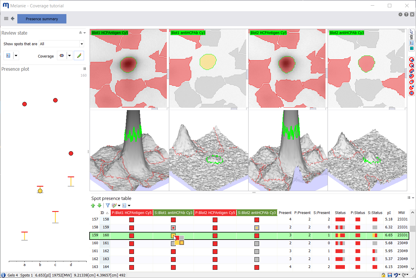
Spot presence table

In the Column settings of the Spot presence table, you can show/hide a number of fields for a color-coded summary of the spot presence states across all images:

• Fields marked P: concern Primary images
• Fields marked S: concern Secondary images
• Present – total number of images on which the spot is present
• P:Present – number of primary images on which the spot is present
• S:Present – number of secondary images on which the spot is present

The three Status fields summarize the spot presence states in a compact way. You can sort the spots based on one of these fields, to select proteins with a similar presence profile.

• Status – summarizes spot presence states for all images
• P:Status – summarizes spot presence states for primary images
• S:Status – summarizes spot presence states for secondary images

A colored square indicates the spot’s presence state on the image, based on the thresholds set in the Presence filter:

• – The spot is Present
• – The spot is Absent
•  – The spot is Uncertain
• – The spot was marked as a Product spot in Spot edition

To edit the presence state of a spot, you can click on the colored square, and pick the desired status: Red, gray or yellow to mark it Present, Absent or Uncertain respectively. The fourth option (lower right) simply indicates the spot’s automatically assigned presence state (based on the thresholds set in the Presence filter step). This fourth option can be red, gray or yellow, depending on what the spot’s automatically assigned presence state was. When you are in Coverage mode, you can also click on a spot in the Display area to modify its presence state.

NOTES

You cannot edit the presence state of Product spots (pink).

When you edit a spot’s presence state, the colored square becomes bi-colored:

• The color of the inner square indicates the spot’s automatically assigned presence state (based on the thresholds set in the Presence filter).
• The color of the outer square indicates the spot’s current/selected presence state.

Please note that the automatically assigned presence state can be changed subsequent to:

• Spot editing; all spots that have undergone editing will appear as uncertain, to make sure you review their presence state.
• Editing of the spot’s coverage status in one of the tabs of the Coverage step.
• Editing of the spot’s presence state in the Presence summary.

Presence plot

The Presence plot lets you review if your coverage status edits are reasonably congruent with the thresholds set in the Presence filter. It shows where each spot’s abundance value (circle) is situated relative to the presence filter thresholds of the corresponding image (represented with gray and red bars delimiting the yellow uncertain interval). The color-coding of the circles in the Presence plot is the same as for the squares in the Spot presence table.

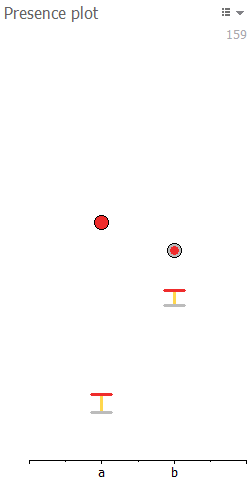
In the Presence plot, the images are ordered according to their appearance in the Display area and labeled with letters on the X-axis. Hover over a label to see the name of the corresponding image. Hover over a circle to see the spot’s abundance value and the filter thresholds that were applied on the particular image.